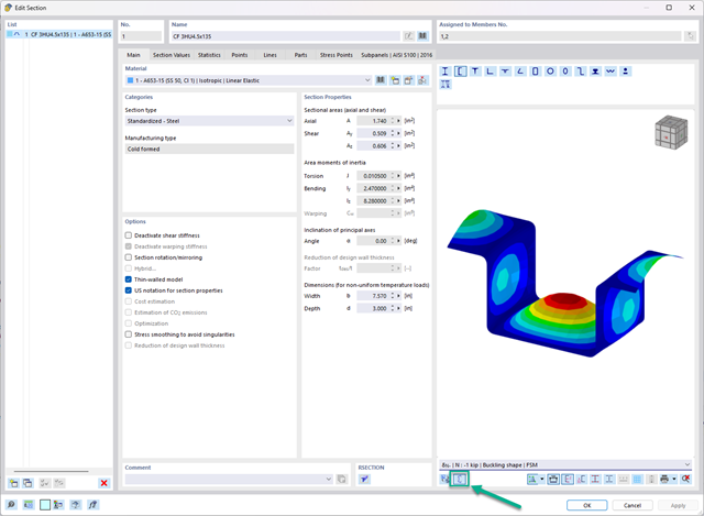
In the "Edit Section" dialog box, you can display the buckling shapes of the Finite Strip Method (FSM) as a 3D graphic.
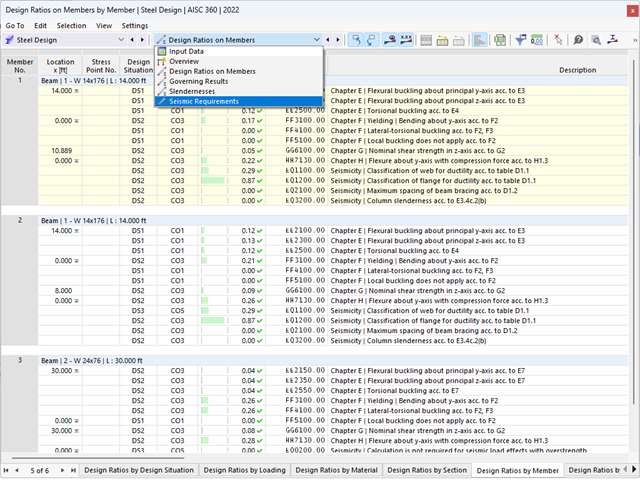
The seismic design result is categorized into two sections: member requirements and connection requirements.
The "Seismic Requirements" include the Required Flexural Strength and the Required Shear Strength of the beam-to-column connection for moment frames. They are listed in the ‘Moment Frame Connection by Member’ tab. For braced frames, the Required Connection Tensile Strength and the Required Connection Compressive Strength of the brace are listed in the ‘Brace Connection by Member’ tab.
The program provides the performed design checks in tables. The design check details clearly display the formulas and references to the standard.

The building model is calculated in two phases:
- Global 3D calculation of the global model, where the slabs are modeled as a rigid plane (diaphragm) or as a bending plate
- Local 2D calculation of the individual floors
After the calculation, the results of the columns and walls from the 3D calculation and the results of the slabs from the 2D calculation are combined in a single model. This means that there is no need to switch between the 3D model and the individual 2D models of the slabs. The user only works with one model, saves valuable time, and avoids possible errors in the manual data exchange between the 3D model and the individual 2D ceiling models.
The vertical surfaces in the model can be divided into shear walls and opening lintels. The program automatically generates internal result members from these wall objects, so they can be designed as members according to any standard in the Concrete Design add-on.
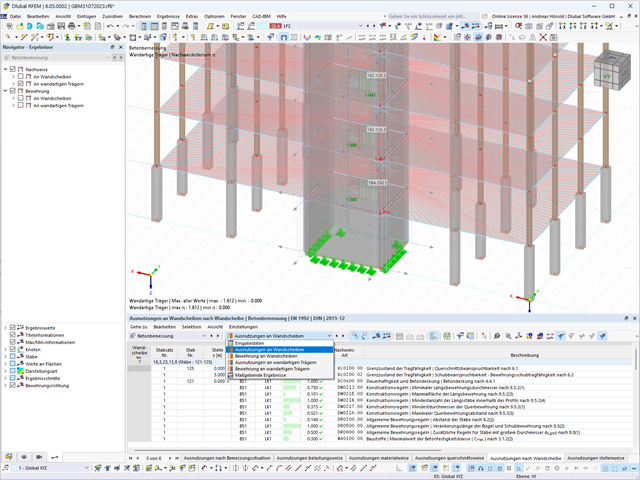
Shear walls and deep beams of a building model are available as independent objects in the design add-ons. This allows for faster filtering of the objects in results, as well as better documentation in the printout report.
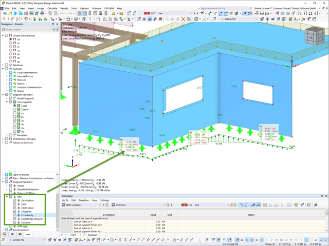
For line support results, you can optionally display certain additional information in info bubbles, such as description, sum, mean value, and so on.
If necessary, you can activate the info bubbles in the Navigator – Results.

The modal relevance factor (MRF) can help you to assess to which extent specific elements participate in a specific mode shape. The calculation is based on the relative elastic deformation energy of each individual member.
The MRF can be used to distinguish between local and global mode shapes. If multiple individual members show significant MRF (for example, > 20%), the instability of the entire structure or a substructure is very likely. On the other hand, if the sum of all MRFs for an eigenmode is around 100%, a local stability phenomenon (for example, buckling of a single bar) can be expected.
Furthermore, the MRF can be used to determine critical loads and equivalent buckling lengths of certain members (for example, for stability design). Mode shapes for which a specific member has small MRF values (for example, < 20%) can be neglected in this context.
The MRF is displayed by mode shape in the result table under Stability Analysis → Results by Members → Effective Lengths and Critical Loads.
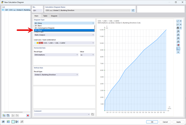
The "2D | Story" calculation diagram type is used to create result diagrams via the building axis. This allows you to easily analyze the behavior of the entire building under static and dynamic effects.
You can use this diagram type, for example, to visualize the seismic force over the building height.
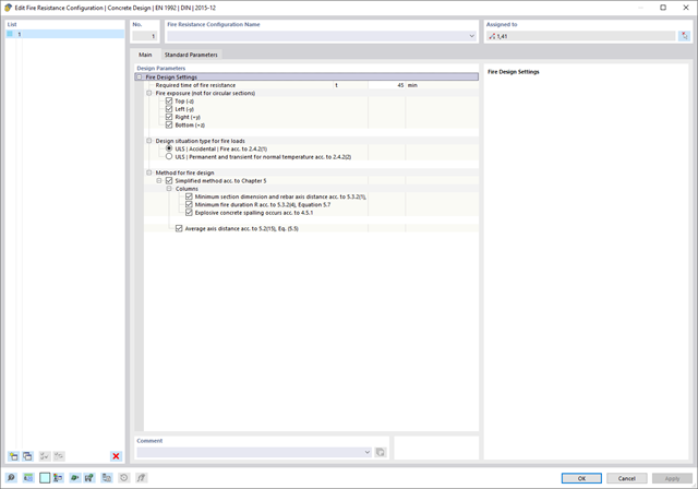
The Concrete Design add-on provides you with the option to perform the simplified fire resistance design according to EN 1992‑1‑2 for columns (Section 5.3.2) and beams (Section 5.6).
The following design checks are available for the simplified fire resistance design:
- Columns: Minimum cross-sectional dimensions for rectangular and circular sections according to Table 5.2a as well as Equation 5.7 for calculating time of fire exposure
- Beams: Minimum dimensions and center distances according to Table 5.5 and Table 5.6
You can determine the internal forces for the fire resistance design according to two methods.
- 1 Here, the internal forces of the accidental design situation are included directly into the design.
- 2 The internal forces of the design at normal temperature are reduced by the factor Eta,fi (ηfi), then used in the fire resistance design.
Furthermore, it is possible to modify the axis distance according to Eq. 5.5.
- Analysis of time diagrams and accelerograms (acceleration-time diagrams exciting the supports of a structure)
- Combination of user-defined time diagrams with nodal, member, and surface loads, as well as free and generated loads
- Combination of several independent excitation functions
- Linear implicit Newmark analysis or modal analysis in time history
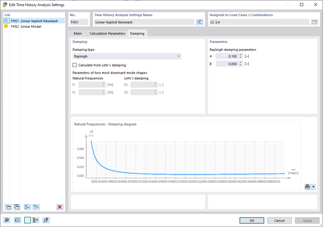
- Structural damping using Raleigh damping coefficients or Lehr's damping value
- Graphical display of results in calculation diagrams
- Result display in individual time steps or as an envelope during the entire time period
- Extensive library of seismic events (accelerograms)
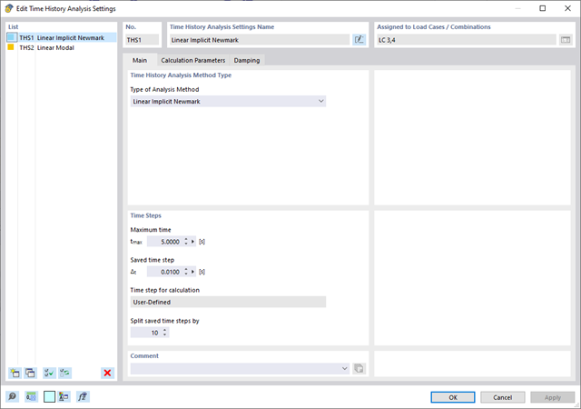
The time history analysis is performed with the modal analysis or the linear implicit Newmark analysis. The time history analysis in this add-on is limited to linear structural systems. Although the modal analysis represents a fast algorithm, it is necessary to use a certain number of eigenvalues to ensure the required accuracy of results.
The implicit Newmark analysis is a very precise method, independent of the number of eigenvalues used, but requires sufficient small time steps for the calculation.
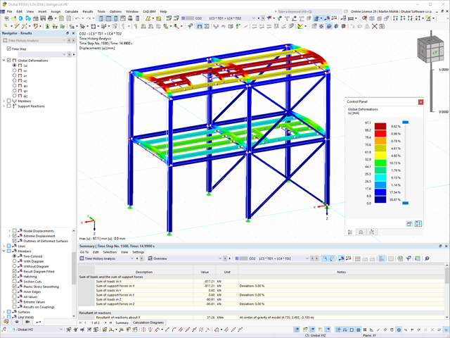
As soon as the program has completed the calculation, the summary of the results is listed. All result windows are integrated in the main program RFEM/RSTAB. You will find all the results arranged in tables; they can be displayed for each individual time step or as an envelope, and you also have the option of displaying the results graphically as well as animating them.
The results from the time history analysis can be displayed in the calculation diagrams. All the results are shown as a function of time. You can export the numeric values to MS Excel.
All result tables and graphics are part of the RFEM/RSTAB printout report. In this way, you can ensure clearly arranged documentation. You can also export the tables to MS Excel.
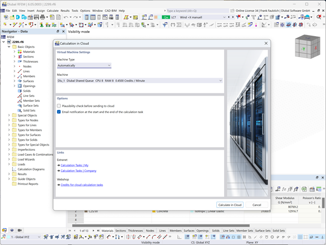
The model and loads are entered as usual in the RFEM interface.
You can start the cloud calculation by selecting an entry in the Calculate menu. Then, select the virtual machine suitable for the task and start the calculation.
After the start, the image is used to create a virtual machine on which the computing server is started. This takes over the calculation of your file.
You can monitor the processing of calculation tasks in the Extranet.
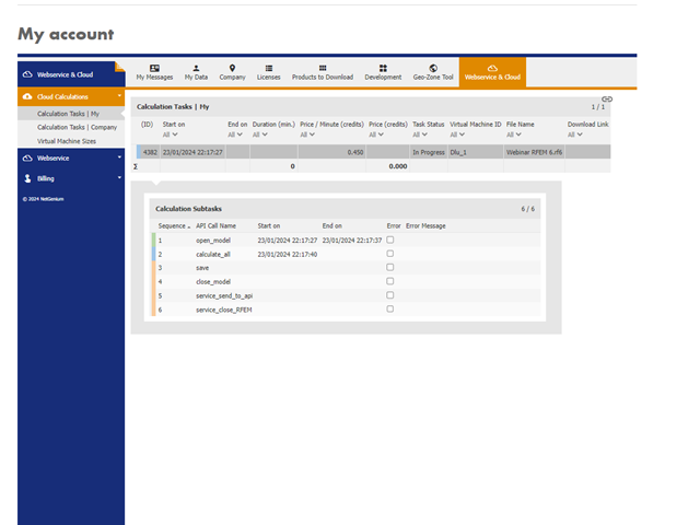
After completing the calculation, you will receive an email with a link to download the calculated file. Large files are compressed into a ZIP archive. Smaller files can be downloaded directly.
As an alternative, there is a link to the calculated file in the Extranet.
The downloaded file is a common RFEM file and can be used for further processing as usual.
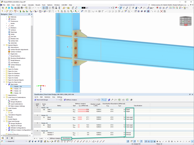
In the Steel Joints add-on, you can classify the joint stiffness.
In addition to the initial stiffness, the table also shows the limit values for hinged and rigid connections for the selected internal forces N, My, and/or Mz. The resulting classification is then displayed in tables as "hinged", "semi-rigid", or "rigid".
Go to Explanatory Video
The Ponding load type allows you to simulate rain actions on multi-curved surfaces, taking into account the displacements according to the large deformation analysis.
This numerical rainfall process examines the assigned surface geometry and determines which rainfall portions drain away and which rainfall portions accumulate in puddles (water pockets) on the surface. The puddle size then results in a corresponding vertical load for the structural analysis.
For example, you can use this feature in the analysis of approximately horizontal membrane roof geometries subjected to rain loading.
Go to Explanatory Video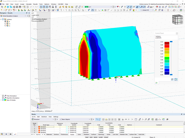
You can display the RWIND results directly in the main program. In the Navigator - Results, select the Wind Simulation Analysis result type from the list above.
Currently, the following results are available, which refer to the RWIND computational mesh:
- Surface pressure
- Surface cp coefficient
- Wall distance y+ (steady flow)
- Consideration of nonlinear component behavior using plastic standard hinges for steel (FEMA 356, EN 1998‑3) and nonlinear material behavior (masonry, steel - bilinear, user-defined working curves)
- Direct import of masses from load cases or combinations for the application of constant vertical loads
- User-defined specifications for the consideration of horizontal loads (standardized to a mode shape or uniformly distributed over the height of the masses)
- Determination of a pushover curve with selectable limit criterion of the calculation (a collapse or limit deformation)
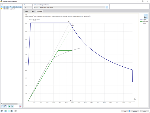
- Transformation of the pushover curve into the capacity spectrum (ADRS format, single degree of freedom system)
- Bilinearization of the capacity spectrum according to EN 1998‑1:2010 + A1:2013
- Transformation of the applied response spectrum into the required spectrum (ADRS format)
- Determination of target displacement according to EC 8 (the N2 method according to Fajfar 2000)
- Graphical comparison of the capacity and required spectrum
- Graphical evaluation of the acceptance criteria of predefined plastic hinges
- Result display of the values used in the iterative calculation of the target displacement
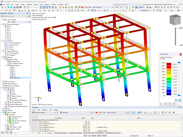
- Access to all results of the structural analysis in the individual load levels
During the calculation, the selected horizontal load is increased in load steps. A static nonlinear analysis is carried out for each load step until reaching the specified limit condition.
The results of the pushover analysis are extensive. On one hand, the structure is analyzed for its deformation behavior. This can be represented by a force-deformation line of the system (a capacity curve). On the other hand, the response spectrum effect can be displayed in the ADRS display (Acceleration-Displacement Response Spectrum). The target displacement is automatically determined in the program based on these two results. The process can be evaluated graphically and in tables.
The individual acceptance criteria can then be graphically evaluated and assessed (for the next load step of the target displacement, but also for all other load steps). The results of the static analysis are also available for the individual load steps.
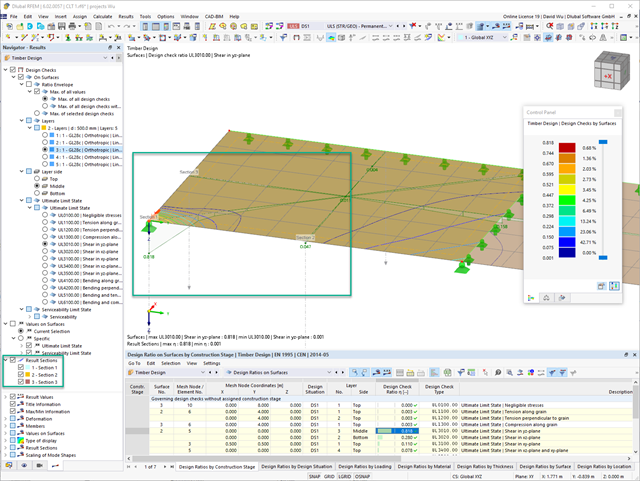
You can graphically evaluate result sections for the timber surface design. This can be done in the RFEM graphic as well as in the result history window. The sections can be placed at any location in order to evaluate the design results in detail.
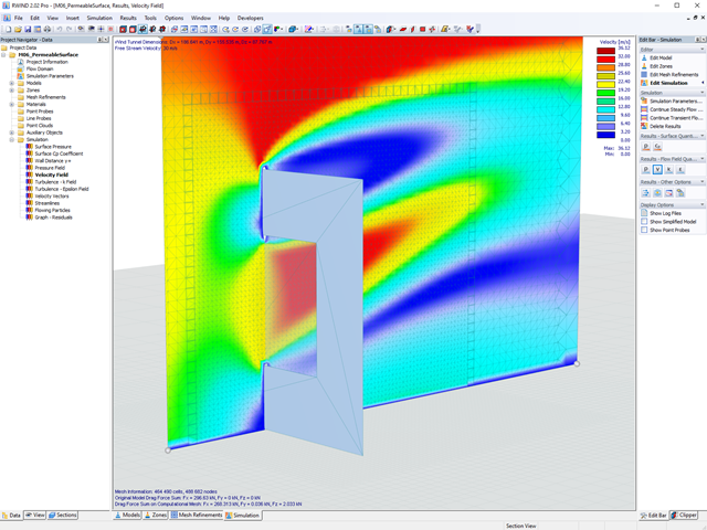
Use RWIND 2 Pro to easily apply a permeability to a surface. All you need is the definition of
- the Darcy coefficient D,
- the inertial coefficient I, and
- the length of the porous medium in the direction of flow L,
to define a pressure boundary condition between the front and back of a porous zone. Due to this setting, you obtain the flow through this zone with a two-part result display on both sides of the zone area.
But that's not all. Furthermore, the generation of a simplified model recognizes permeable zones and takes into account the corresponding openings in the model coating. Can you waive an elaborate geometric modeling of the porous element? Understandable – we have good news for you then! With a pure definition of the permeability parameters, you can avoid complex geometric modeling of the porous element. Use this feature to simulate permeable scaffolding, dust curtains, mesh structures, and so on.
More Information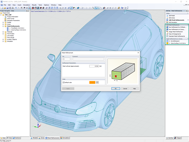
Do you already know the editor for mesh refinement control? It is a great help for your work! Why? It's easy – it gives you the following options:
- Graphic visualization of the areas with mesh refinements
- Mesh refinement of zones
- Deactivating the standard 3D solid mesh refinement with transversion into the corresponding manual 3D mesh refinements.
These options help you to formulate a suitable rule for meshing the entire model, even for the models with unusual dimensions. Use the editor to efficiently define small model details on large buildings or detailed meshing areas in the coating area of the model. You will be amazed!
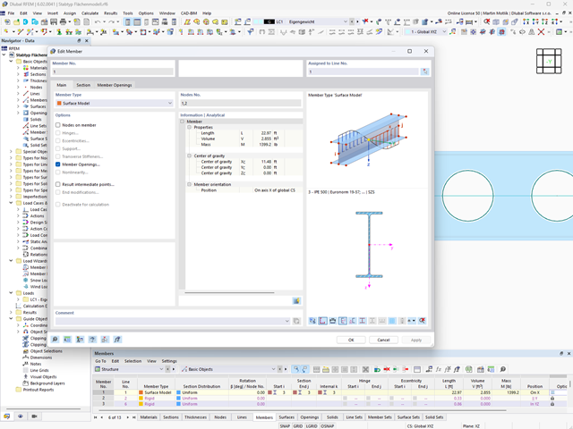
Can you use some support? The "surface model" member type helps you to simulate a member as a surface model in the overall model.
This feature provides you with the following:
- Quick input using a member with a cross-section
- Simulation of openings in the web
- Simultaneous output of the member and surface results
- Design of member results in the add-on
- Consideration of a real stress distribution
You can use the surface member for the following applications, among others:
- Castellated beams
- Perforated beams
- Beams with rectangular openings
- Vierendeel trusses
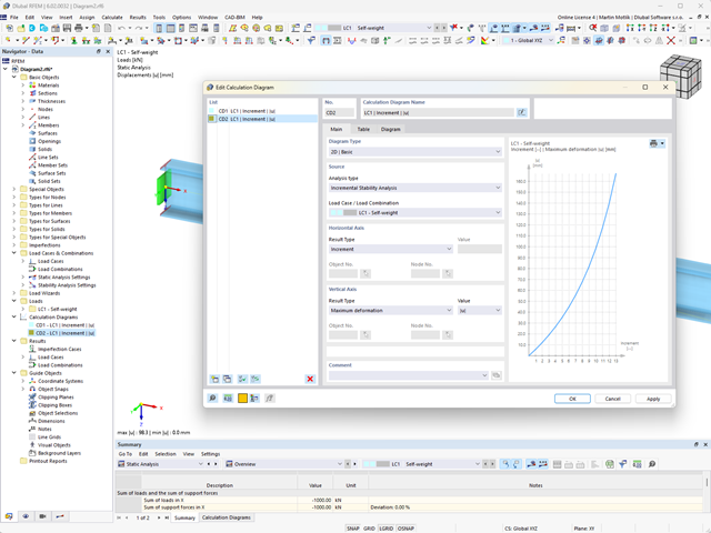
Do you want to create calculation diagrams? With RFEM and RSTAB, this works globally and without any problems. Create and organize your calculation diagrams directly in the Navigator - Data or via the menu Insert → Calculation Diagrams.
Use calculation diagrams to record and display a relation between the various calculation results.
It is also possible to superimpose similar diagrams.
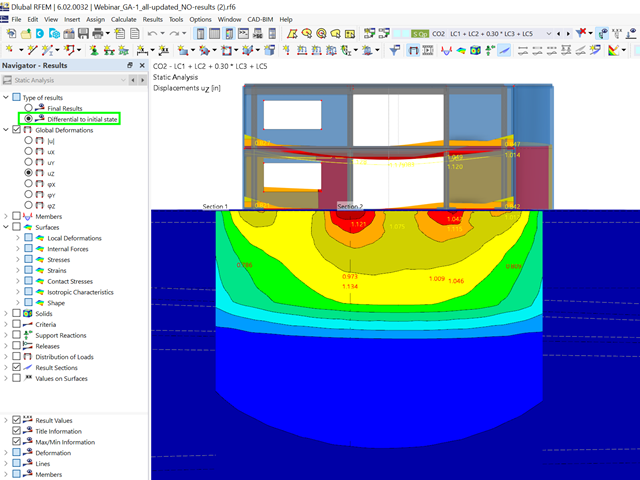
Did you already know? For load combinations, you can optionally display the difference results to the initial state. For example, you have the option for a geotechnical analysis to output the settlement as a difference to the initial state "soil self-weight".
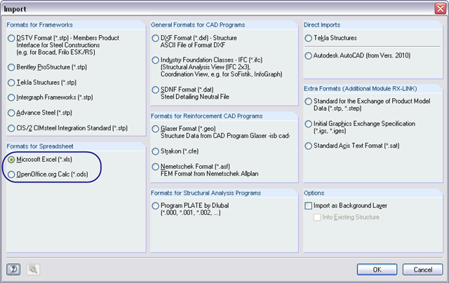
You can import table values from a prepared Excel table into RFEM 6 / RSTAB 9 with just a few clicks – either individually or all at once. For the import, you need to install a plug-in in Microsoft Excel according to this FAQ.
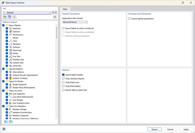
Did you know? You can export all RFEM/RSTAB tables with the results individually or all at once directly into an Excel table or as a CSV file. There are several options available to you:
- With table headers
- Selected objects only
- Filled rows only
- Only filled tables
- Export data as plain text
This way, the program allows you to control and clearly manage the exported data. You can export the stored formulas directly in the table or as a separate table, as in the case of the used parameters.
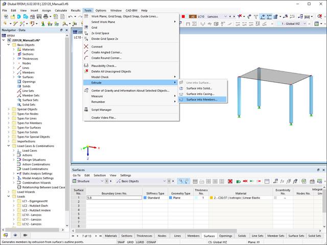
Did you know that you can extrude surfaces into members? In this case, the program assigns a desired member property to the lines generated by the extrusion. A few clicks later, you are already at the desired result.
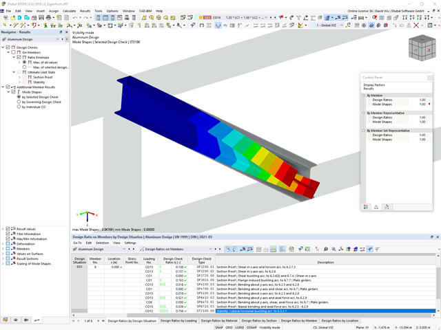
Did you use the eigenvalue solver of the add-on to determine the critical load factor within the stability analysis? In this case, you can then display the governing mode shape of the object to be designed as a result.
.png?mw=640&hash=55038d2a1591f62179796666cb9b2fede0274e19)
A graphical and tabular output of the results for deformations, stresses, and strains helps you when determining the soil solids. To achieve this, use the special filter criteria for targeted selection of results.
The program doesn't leave you alone with the results. If you want to graphically evaluate the results in the soil solids, you can use the guide objects. For example, you can define clipping planes. This allows you to view the corresponding results in any plane of the soil solid.
And not just that. The utilization of result sections and clipping boxes facilitates the precise graphical analysis of the soil solid.
You already know that it is possible to model and analyze a soil and a structure in the entire model. As a result, you have explicitly taken into account the soil-structure interaction. By modifying a component, you achieve the immediate correct consideration in the analysis as well as in the results for the entire system of the soil and structure.